What Is The Sample Size In A Two Factor Anova

Two-style ANOVA | When and How to Utilise it, With Examples

Published on March 20, 2020 past Rebecca Bevans. Revised on January 7, 2021.

ANOVA (Analysis of Variance) is a statistical examination used to analyze the difference between the means of more ii groups.

A two-way ANOVA is used to gauge how the mean of a quantitative variable changes according to the levels of 2 categorical variables. Utilize a two-style ANOVA when you desire to know how two independent variables, in combination, affect a dependent variable.

Instance

Yous are researching which type of fertilizer and planting density produces the greatest crop yield in a field experiment. Yous assign different plots in a field to a combination of fertilizer type (i, 2, or 3) and planting density (ane=depression density, 2=high density), and measure the last crop yield in bushels per acre at harvest time.

You lot can use a two-mode ANOVA to find out if fertilizer type and planting density have an result on average crop yield.

When to use a ii-mode ANOVA

You can use a two-fashion ANOVA when you have collected data on a quantitative dependent variable at multiple levels of two categorical independent variables.

A quantitative variable represents amounts or counts of things. It can exist divided to find a grouping mean.

Bushels per acre is a quantitative variable considering it represents the amount of ingather produced. Information technology tin be divided to detect the average bushels per acre.

A chiselled variable represents types or categories of things. A level is an private category inside the categorical variable.

Fertilizer types one, 2, and 3 are levels within the categorical variablefertilizer type. Planting densities 1 and two are levels inside the categorical variable planting density.

You lot should have plenty observations in your information gear up to exist able to detect the mean of the quantitative dependent variable at each combination of levels of the contained variables.

Both of your independent variables should be categorical. If one of your contained variables is categorical and 1 is quantitative, use an ANCOVA instead.

How does the ANOVA test work?

ANOVA tests for significance using the F-test for statistical significance. The F-examination is a groupwise comparison examination, which means it compares the variance in each group mean to the overall variance in the dependent variable.

If the variance within groups is smaller than the variance between groups, the F-examination will find a higher F-value, and therefore a higher likelihood that the difference observed is real and not due to chance.

A two-mode ANOVA with interaction tests three zip hypotheses at the same time:

At that place is no deviation in grouping means at any level of the offset independent variable.
There is no departure in group means at any level of the 2d independent variable.
The issue of one independent variable does not depend on the upshot of the other independent variable (a.k.a. no interaction upshot).

A two-way ANOVA without interaction (a.k.a. an additive 2-mode ANOVA) only tests the get-go ii of these hypotheses.

Two-style ANOVA hypotheses

In our crop yield experiment, we can examination iii hypotheses using two-way ANOVA:

Null hypothesis (H₀)	Alternate hypothesis (H_a)
At that place is no difference in average yield for any fertilizer type.	There is a departure in average yield by fertilizer type.
There is no divergence in average yield at either planting density.	There is a difference in boilerplate yield by planting density.
The effect of one independent variable on boilerplate yield does not depend on the upshot of the other contained variable (a.chiliad.a. no interaction effect).	There is an interaction consequence between planting density and fertilizer blazon on average yield.

What is your plagiarism score?

Compare your paper with over threescore billion web pages and 30 million publications.

Best plagiarism checker of 2021
Plagiarism study & percentage
Largest plagiarism database

Scribbr Plagiarism Checker

Assumptions of the ii-way ANOVA

To use a two-way ANOVA your data should run into certain assumptions.Two-manner ANOVA makes all of the normal assumptions of a parametric test of difference:

Homogeneity of variance (a.yard.a. homoscedasticity)

The variation around the hateful for each group being compared should be similar among all groups. If your data don't encounter this assumption, yous may be able to use a not-parametric alternative, like the Kruskal-Wallis test.

Independence of observations

Your independent variables should non be dependent on one some other (i.e. ane should not cause the other). This is impossible to test with categorical variables – information technology can just be ensured past good experimental design.

In addition, your dependent variable should stand for unique observations – that is, your observations should not exist grouped within locations or individuals.

If your information don't meet this assumption (i.e. if you lot set up experimental treatments within blocks), you tin can include a blocking variable and/or use a repeated-measures ANOVA.

Normally-distributed dependent variable

The values of the dependent variable should follow a bell curve. If your data don't meet this assumption, you lot can endeavour a data transformation.

In the ingather-yield example, the response variable is normally distributed, and we can check for homoscedasticity after running the model. The experimental treatments were gear up up within blocks in the field, with four blocks each containing every possible combination of fertilizer type and planting density, so nosotros should include this as a blocking variable in the model.

How to perform a two-fashion ANOVA

The dataset from our imaginary crop yield experiment includes observations of:

Last ingather yield (bushels per acre)
Type of fertilizer used (fertilizer type i, two, or three)
Planting density (1=depression density, 2=high density)
Block in the field (ane, 2, three, four).

The 2-style ANOVA will test whether the contained variables (fertilizer type and planting density) have an consequence on the dependent variable (average crop yield). But there are some other possible sources of variation in the information that we want to have into account.

We practical our experimental treatment in blocks, then we desire to know if planting block makes a departure to average ingather yield. We besides want to check if there is an interaction consequence between 2 contained variables – for example, it'due south possible that planting density affects the plants' ability to take upward fertilizer.

Because we have a few different possible relationships betwixt our variables, we will compare three models:

A 2-style ANOVA without whatsoever interaction or blocking variable (a.k.a an additive two-way ANOVA).
A two-fashion ANOVA with interaction but with no blocking variable.
A two-way ANOVA with interaction and with the blocking variable.

Model one assumes there is no interaction between the two independent variables. Model 2 assumes that in that location is an interaction betwixt the two contained variables. Model 3 assumes there is an interaction betwixt the variables, and that the blocking variable is an important source of variation in the information.

By running all 3 versions of the two-mode ANOVA with our data then comparing the models, we can efficiently test which variables, and in which combinations, are of import for describing the data, and see whether the planting block matters for average crop yield.

This is not the only manner to do your analysis, but it is a good method for efficiently comparing models based on what y'all think are reasonable combinations of variables.

Running a two-way ANOVA in R

We will run our analysis in R. To try it yourself, download the sample dataset.

Sample dataset for a two-way ANOVA

After loading the data into the R environs, we will create each of the three models using the aov() control, and so compare them using the aictab() command. For a full walkthrough, meet our guide to ANOVA in R.

This first model does not predict any interaction between the contained variables, so we put them together with a '+'.

Two-style ANOVA R code

2.way <- aov(yield ~ fertilizer + density, data = crop.data)

In the 2nd model, to test whether the interaction of fertilizer type and planting density influences the last yield, apply a ' * ' to specify that you also want to know the interaction effect.

Two-style ANOVA with interaction R code

interaction <- aov(yield ~ fertilizer * density, data = ingather.data)

Because our ingather treatments were randomized within blocks, we add this variable equally a blocking cistron in the tertiary model. Nosotros can then compare our 2-way ANOVAs with and without the blocking variable to encounter whether the planting location matters.

Two-style ANOVA with blocking R code

blocking <- aov(yield ~ fertilizer * density + block, data = crop.data)

Model comparison

Now nosotros tin can find out which model is the all-time fit for our information using AIC (Akaike information criterion) model choice.

AIC calculates the all-time-fit model by finding the model that explains the largest corporeality of variation in the response variable while using the fewest parameters. Nosotros tin can perform a model comparison in R using the aictab() office.

AIC R code

                  library(AICcmodavg)  model.set <- list(two.way, interaction, blocking) model.names <- c("two.way", "interaction", "blocking")  aictab(model.gear up, modnames = model.names)

The output looks like this:

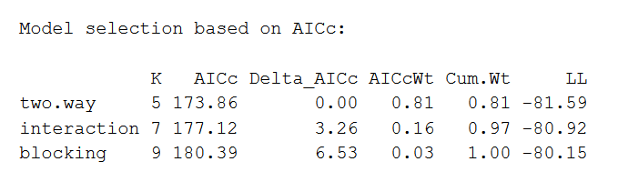
AIC model selection table, with best model listed first

The AIC model with the best fit volition be listed first, with the second-best listed next, and then on. This comparison reveals that the ii-way ANOVA without whatever interaction or blocking effects is the best fit for the data.

Interpreting the results of a ii-style ANOVA

Y'all can view the summary of the two-way model in R using the summary() command. We will accept a look at the results of the first model, which we found was the best fit for our data.

Two-style ANOVA summary R code

summary(two.style)

The output looks like this:

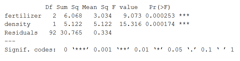
Model summary of a two-way ANOVA without interaction in R.

The model summary starting time lists the independent variables beingness tested ('fertilizer' and 'density'). Next is the rest variance ('Residuals'), which is the variation in the dependent variable that isn't explained past the independent variables.

The post-obit columns provide all of the information needed to interpret the model:

Df shows the degrees of liberty for each variable (number of levels in the variable minus 1).
Sum sq is the sum of squares (a.k.a. the variation between the group ways created by the levels of the contained variable and the overall mean).
Mean sq shows the mean sum of squares (the sum of squares divided past the degrees of freedom).
F value is the test statistic from the F-test (the hateful foursquare of the variable divided past the mean square of each parameter).
Pr(>F) is the p-value of the F statistic, and shows how likely it is that the F-value calculated from the F-test would have occurred if the null hypothesis of no deviation was true.

From this output we tin can meet that both fertilizer type and planting density explicate a significant amount of variation in average crop yield (p-values < 0.001).

Post-hoc testing

ANOVA volition tell you which parameters are significant, but not which levels are actually unlike from i another. To test this we tin can employ a post-hoc test. The Tukey's Honestly-Significant-Divergence (TukeyHSD) test lets us run into which groups are dissimilar from one another.

Tukey R code

TukeyHSD(ii.mode)

The output looks like this:

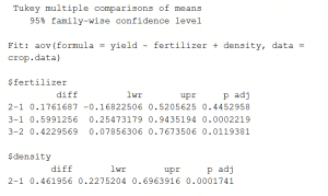
Summary of a TukeyHSD post-hoc comparison for a two-way ANOVA in R.

This output shows the pairwise differences between the three types of fertilizer ($fertilizer) and betwixt the two levels of planting density ($density), with the average difference ('diff'), the lower and upper bounds of the 95% confidence interval ('lwr' and 'upr') and the p-value of the difference ('p-adj').

From the post-hoc test results, we come across that there are significant differences (p < 0.05) between:

fertilizer groups 3 and 1,
fertilizer types 3 and 2,
the 2 levels of planting density,

but no divergence between fertilizer groups two and 1.

How to present the results of a a two-fashion ANOVA

Once you have your model output, you lot tin can report the results in the results section of your paper.

When reporting the results you should include the f-statistic, degrees of freedom, and p-value from your model output.

Case results

We plant a statistically-pregnant difference in average corn yield past both fertilizer type (f(2)=nine.018, p < 0.001) and by planting density (f(1)=15.316, p<0.001), though the interaction between these terms was not significant.

A Tukey postal service-hoc test revealed meaning pairwise differences betwixt fertilizer mix three and fertilizer mix i (+ 0.59 bushels/acre under mix 3), between fertilizer mix iii and fertilizer mix two (+ 0.42 bushels/acre under mix 2), and between planting density 2 and planting density one ( + 0.46 bushels/acre under density 2).

You lot tin can talk over what these findings mean in the discussion section of your paper.

Example discussion

The increased production under fertilizer mix 3 and at higher planting densities suggests that under field conditions similar to ours, this combination would be well-nigh advantageous for crop yield. The lack of interaction between fertilizer blazon and planting densities suggests that planting density does not affect the ability of the plants to take upward fertilizer, though at densities higher than ours this may become the case.

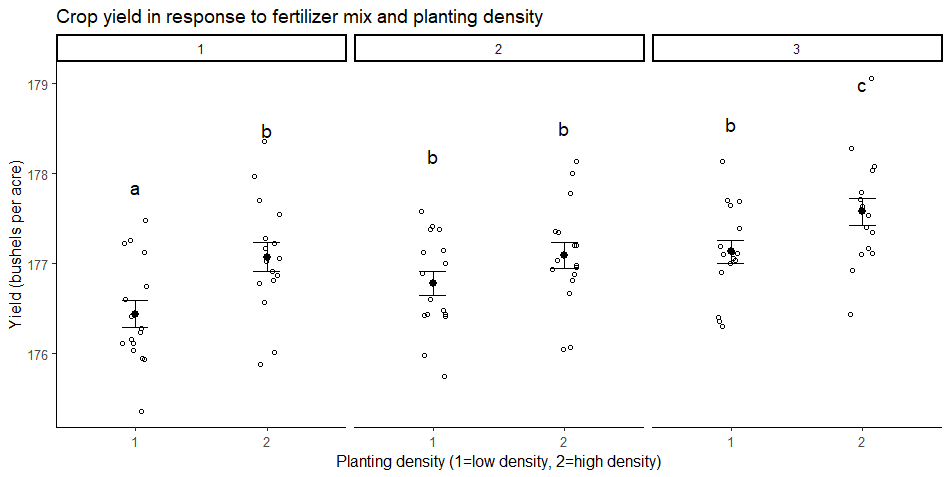
You lot may likewise desire to brand a graph of your results to illustrate your findings.

Your graph should include the groupwise comparisons tested in the ANOVA, with the raw information points, summary statistics (represented here every bit means and standard error bars), and letters or significance values to a higher place the groups to show which groups are significantly unlike from the others.

Groupwise comparisons graph illustrating the results of a two-way ANOVA.

Oft asked questions about ii-way ANOVA

What is the difference between a one-fashion and a two-way ANOVA?: The only departure between one-manner and two-way ANOVA is the number of independent variables. A one-style ANOVA has one contained variable, while a 2-mode ANOVA has two.

One-way ANOVA: Testing the human relationship between shoe make (Nike, Adidas, Saucony, Hoka) and race finish times in a marathon.

Two-way ANOVA: Testing the human relationship betwixt shoe brand (Nike, Adidas, Saucony, Hoka), runner age group (junior, senior, master'south), and race finishing times in a marathon.

All ANOVAs are designed to test for differences amongst 3 or more than groups. If yous are only testing for a divergence between ii groups, use a t-test instead.
How is statistical significance calculated in an ANOVA?: In ANOVA, the cipher hypothesis is that in that location is no difference among group means. If whatever group differs significantly from the overall group mean, then the ANOVA will report a statistically meaning result.

Significant differences amid grouping means are calculated using the F statistic, which is the ratio of the hateful sum of squares (the variance explained past the independent variable) to the mean square error (the variance left over).

If the F statistic is higher than the critical value (the value of F that corresponds with your alpha value, commonly 0.05), then the deviation among groups is accounted statistically significant.
What is a factorial ANOVA?: A factorial ANOVA is any ANOVA that uses more than 1 categorical independent variable. A two-mode ANOVA is a type of factorial ANOVA.

Some examples of factorial ANOVAs include:

Testing the combined effects of vaccination (vaccinated or not vaccinated) and health condition (good for you or pre-existing condition) on the rate of influenza infection in a population.

Testing the effects of marital status (married, single, divorced, widowed), job status (employed, self-employed, unemployed, retired), and family history (no family history, some family history) on the incidence of depression in a population.

Testing the effects of feed blazon (blazon A, B, or C) and barn crowding (non crowded, somewhat crowded, very crowded) on the concluding weight of chickens in a commercial farming operation.
What is the difference between quantitative and categorical variables?: Quantitative variables are whatever variables where the information correspond amounts (e.thousand. elevation, weight, or age).

Categorical variables are whatever variables where the data stand for groups. This includes rankings (due east.g. finishing places in a race), classifications (e.g. brands of cereal), and binary outcomes (e.thousand. coin flips).

You demand to know what type of variables you lot are working with to choose the right statistical test for your data and interpret your results.

Is this commodity helpful?

You have already voted. Cheers :-) Your vote is saved :-) Processing your vote...